Purpose
|
|
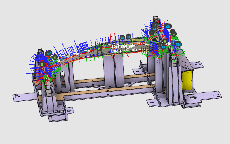
After setting up the workcell with the parts that are going to be processed, the laser cut programs can be generated, optimized and simulated.
|
|
|
The cutting contours will be programmed in separated groups with different strategies. Examples will show how the computed toolpaths can be modified using the manual teach capabilities, changing attribute values, and recalculating the toolpath with interpolation algorithms.
The results can then be simulated.
|
|
|
Steps
|
|

|
Be sure to save your changes frequently.
|
|
|
1
|
Preparation
|
1.1
|

|
Verify the project setup. The tool frame should be located at the focal point of the laser beam. The base frame represents the origin of your new program. A new base frame will be created on the fixture.
|
|
1.2
|

|
Create a new, empty program.
|
|
|
2
|
Program the toolpaths
|
Plan the sequence to cut the inner contours in a smart way to reduce unnecessary laser head movements.
|
2.1
|

|
Create the first group of operation: Hold the CTRL key and select the first three contours to program the process geometries.
|
|
2.2
|

|
Use the Display filter to enhance the view.
|
|
2.3
|
|
The generated toolpath can be modified, i.e. start position, approach direction, etc.
|
|
2.4
|

|
Modify the attributes that are applied to program the toolpath. Many different attributes are being used to compute the toolpath, such as approximation algorithms, singularity optimization, approach and retract strategies, etc.
|
|
|
3
|
Organize the operations
|
|
3.1
|
|
View the structure of the active program.
|
|
3.2
|

|
Simulate the program (partially) to get a first impression.
|
|
3.3
|
|
Program the other toolpath groups on the workpiece.
|
|
3.4
|
|
If needed, optimize the order of cutting operations within the operation group in such a logical sequence to have smooth machine motion and to avoid unnecessary runs.
|
|
1
|
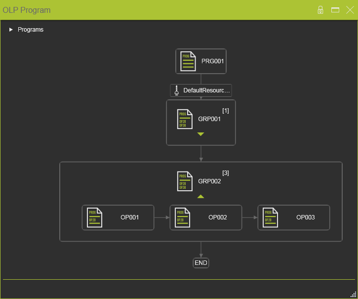
Start the Active Program dashboard by picking the icon in the right dashboard toolbar.
|

|
|
|
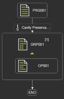
The dashboard window appears, showing a graphical flow of the program with all operation groups.
|
|
|
2
|
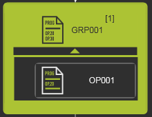
Pick an operation within a group to make it active.
|
|
|
|
The mouse switches to move behavior.
|
|
|
3
|
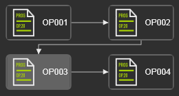
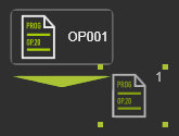
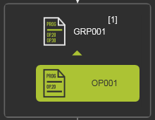
The operation graphics now can be dragged away.
|

|
|
4
|
Dragging the operation to the top of another one inserts it in front of this receiving operation.
|
|
|
5
|
Or dragging the operation to the bottom of another one inserts it behind this receiving operation.
|
|
|
|
|
|
3.5
|
|
Give appropriate names to the operation group and individual operations.
|
|
1
|
Start the Active Program dashboard by picking the icon in the right dashboard toolbar.
|
|
|
The dashboard window appears. In the graphics is displayed from top to bottom, the program and the operation group with its individual operations.
|
|
2
|
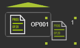
Pick the program graphic to activate it. It will be highlighted.
|

|
3
|
Pick the program name to start the editor. Modify the name.
The modification is executed on the fly; leaving the name field, or any other activity, automatically confirms the new name.
|

|
4
|
With the same procedure the name of the operation group and of the individual operations can be edited.
|
|
|
|
|
|
4
|
Fine tuning the operations: events and teaching
|
|
Using manual teach functionality to fine-tune the operations and transitions between the operations.
|
|
Different functions, strategies and optimization algorithms are available. A few of them are described here.
|
4.1
|

|
Change to the Events and teach work environment.
|
4.2
|
|
Interpolation of the toolpath normal vectors.
|
|
4.3
|

|
Optimize the circle toolpath orientation.
|
|
|
|
4.5
|
|
Modify the toolpath local approach and retract steps to minimize the laser head motion.
|
|
4.6
|
|
To improve the toolpath, for example to avoid collision, additional positions can be inserted.
|
|
4.7
|
|
Define an event to open the clamp of the fixture.
|
|
|
|
4.9
|
|
Optimize the C-axis motion of the machine with intelligent interpolation functionality that automatically locks the motion of the other head axes.
 Example 1 Example 1
Example 2
|
|
4.10
|
|
Add contour offsets.
|
|
4.11
|
|
Add different technology events.
|
|
|
|
|
5.1
|
|
Simulate the complete program.
|
|
|
|
|
|
6.1
|
|
Verify the technology table.
|
|
|
|
|
7.1
|

|
Save the project under an appropriate name.
|
|
1
|
Start the Save Project command by picking the icon with the left mouse button.
|
|
2
|
A windows file browser appears.
|
|
3
|
Browse to the disk and folder where the project needs to be stored.
|
|
4
|
Accept the default proposed name of the project or change it when necessary.
|

|
5
|
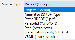
In the option Save as type select the document format in which the project has to be stored.
|
|
6
|
Confirm saving the project by clicking on the Save button.
|

|
|
|
|
|
|

